Predicting Employee Turnover — a practical, interpretable pipeline

This post describes a compact, reproducible pipeline I used to predict employee turnover on a small, real-world HR dataset (1.1K rows). The goal was not just to maximize a metric but to produce an interpretable model that helps guide retention interventions.

Below you’ll find the dataset summary, preprocessing steps, model comparisons, and concrete takeaways. The notebook used to produce these results (data cleaning, full grid-search, and figures) is available in this GitHub repository.

---

Dataset

I used the Kaggle dataset davinwijaya/employee-turnover (1,129 rows × 16 columns). There are no missing values. The target column is event (turnover indicator). The remaining columns include demographics, hiring channel information, salary characteristics, and several psychometric trait scores. Important columns:

• stag — tenure / experience (time)
• event — target (employee turnover)
• gender — f / m
• age — employee age (years)
• industry, profession — categorical job descriptors
• traffic — recruitment channel (multi-class)
• coach — presence of onboarding/training coach
• head_gender — manager/supervisor gender
• greywage — unofficial (partially off-record) salary component
• way — commute / transportation method
• Psychometric scores: extraversion, independ, selfcontrol, anxiety, novator

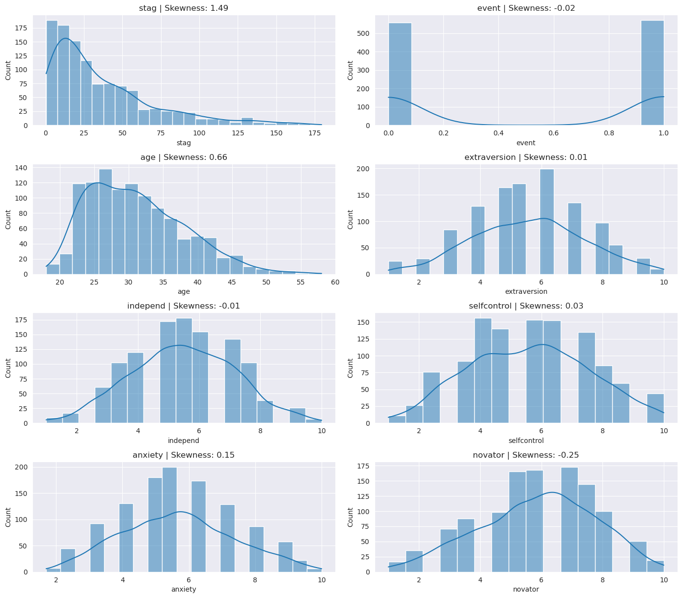
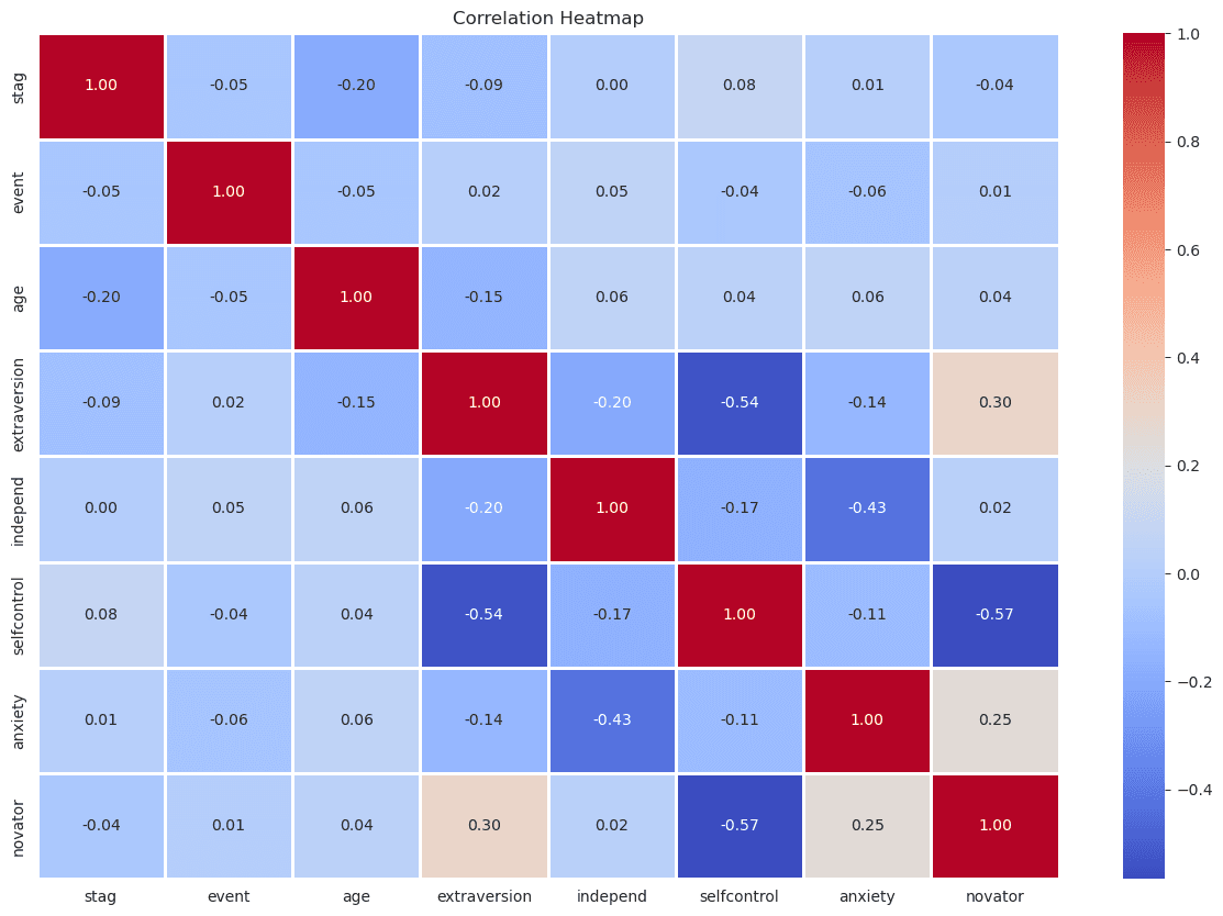
I included an exploratory figure (histograms, KDEs and a correlation heatmap) to check distributions and pairwise relationships. The most notable pattern was weak negative correlation among selfcontrol, anxiety, and novator.

Preprocessing

• Label-encoded binary columns and one-hot encoded multi-class columns (drop first level to avoid collinearity).
• Resulting feature matrix: 50 features.
• Standardized numeric features with StandardScaler.
• Train/test split: 80/20 (train 903×50, test 226×50), stratified on the target.

This preprocessing pipeline was implemented in the notebook so experiments can be reproduced exactly.

---

Modeling approach and evaluation

I compared several models with standard scikit-learn workflows: logistic regression (regularized), Random Forest, a small feedforward neural network, XGBoost, and Gradient Boosting. For hyperparameter tuning I used grid search with cross-validation (typically 4–5 folds) and F1/accuracy metrics where appropriate.

Primary evaluation metrics reported here are test accuracy and macro F1 (when class balance matters). Where I report a single F1/accuracy value below, that is measured on the held-out test set using the best hyperparameters selected via cross-validation.

Logistic regression

• Implementation: LogisticRegression(max_iter=1000)
• Grid search over C, penalty, and solver (5-fold CV, F1 scoring)
• Result: Test accuracy ≈ 0.67, F1 ≈ 0.67. Best params: C=0.01, penalty='l1', solver='saga'.

The linear baseline performed respectably but underfit compared with tree-based models.

Random Forest (interpretable ensemble)

• Baseline: 100 trees.
• Hyperparameter search (grid): n_estimators, max_depth, min_samples_split.
• Best configuration after grid search: n_estimators=50, max_depth=10, min_samples_split=2.
• Test performance: accuracy ≈ 0.73; F1 ≈ 0.74 (held-out test set).

Feature importances were computed from the trained Random Forest and used both to explain the model and to evaluate a reduced-feature experiment (top-N features). The top predictors were: stag, age, independ, selfcontrol, novator, anxiety, and extraversion.

Plot: feature importances reshaped to 28×28 for visual inspection (see notebook). A reduced model using only the top 15 features decreased F1 to ≈ 0.63, so the full feature set performed better in this case.

Neural network (small MLP)

• Architecture: single hidden layer (32 units, ReLU), dropout 0.2, sigmoid output.
• Optimizer: Adam (lr=0.001). Loss: BCEWithLogitsLoss.
• Training: 70/30 train/validation split with early stopping.
• Result: Training F1 reached ≈ 0.74, but test F1 dropped to ≈ 0.64 — clear overfitting given limited data.

XGBoost / Gradient Boosting

• XGBoost (binary:logistic) with default settings and some tuning returned test accuracy ≈ 0.69 / F1 ≈ 0.70. Gradient Boosting was comparable after lightweight hyperparameter search. Tree-based ensembles were the best compromise of predictive performance and interpretability.

---

Takeaways

• For this modest (~1.1K rows) tabular dataset, classical tree ensembles (Random Forest, XGBoost) generalized best and produced useful feature importance measures.
• Logistic regression underperformed compared to trees, while the neural network overfit despite regularization and early stopping — a reminder that deep models need substantially more data or stronger regularization to win.
• The most consistent predictors of turnover were tenure (stag), age, and personality metrics (independ, selfcontrol, novator, anxiety, extraversion). These align with practical intuition: both tenure and individual traits matter.

Recommendations

If this model were to be used operationally inside a company, I recommend:

1. Use model outputs as signals, not actions: flag high-risk employees for human review and supportive interventions (coaching, career development conversations, compensation review).
2. Keep transparency and consent: communicate clearly how the model is used and ensure fairness checks (disparate impact by gender/age/etc.).
3. Monitor model drift: retrain periodically as hiring channels and business context change.